
A Data Engineer’s Guide to Vector Databases (Part 1): Core Concepts Before Building AI-Powered Applications
A practical foundation for data engineers transitioning from relational to vector-based data systems.

As data engineers, we’re all familiar with relational databases, SQL queries, and structured schemas. We know how to efficiently store, join, and retrieve data. But as AI systems and unstructured data become central to modern applications, traditional databases start to show their limitations, especially when the questions we ask aren’t exact matches, but semantic in nature.
In this post, we’ll introduce vector databases and break down six core concepts every data engineer should understand before using them for AI-powered applications:
Embeddings
Dimensionality
Chunking
Similarity Scoring
Ranking and Reranking
Search Modes
In part two, we’ll get hands-on to build a vector database, apply these concepts, and see them in action on a real dataset.
What is a Vector Database

Before diving into vector databases, it’s helpful to first revisit what a database is and what we mean by a vector. Once we understand these two concepts individually, we can see what happens when they come together.
Database
A database is essentially an organised digital filing system for information. It collects related data (such as names, addresses, numbers, or product details) and stores it together so a computer can manage it. We can think of a database like a well-organised library: it keeps everything in order, allowing us to store, retrieve, and update information easily. In simple terms, a database helps us keep a large amount of data in one place and find specific items quickly.
Most traditional databases, primarily relational databases1, use Structured Query Language (SQL)2 to manage and manipulate stored data. Traditional databases are excellent at answering precise, fact-based queries such as:
“Find the book where the description is ‘DevOps’.”
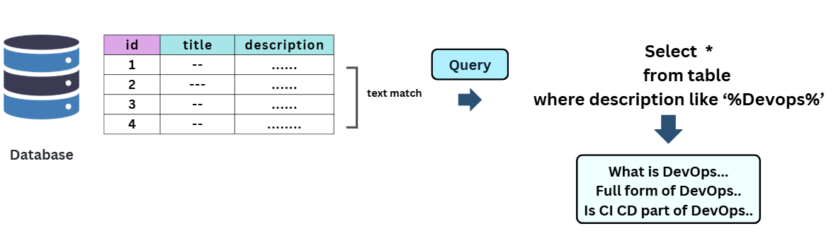
However, they struggle when queries become more fuzzy or semantic, like:
“Find books that explain modern DevOps practices or are similar to the DevOps Handbook.” (we might use couple of SQL LIKE Operator for each word and got nothing.)
That’s because traditional databases rely on exact keyword matches or fixed rules, not on understanding the meaning or context of the data.
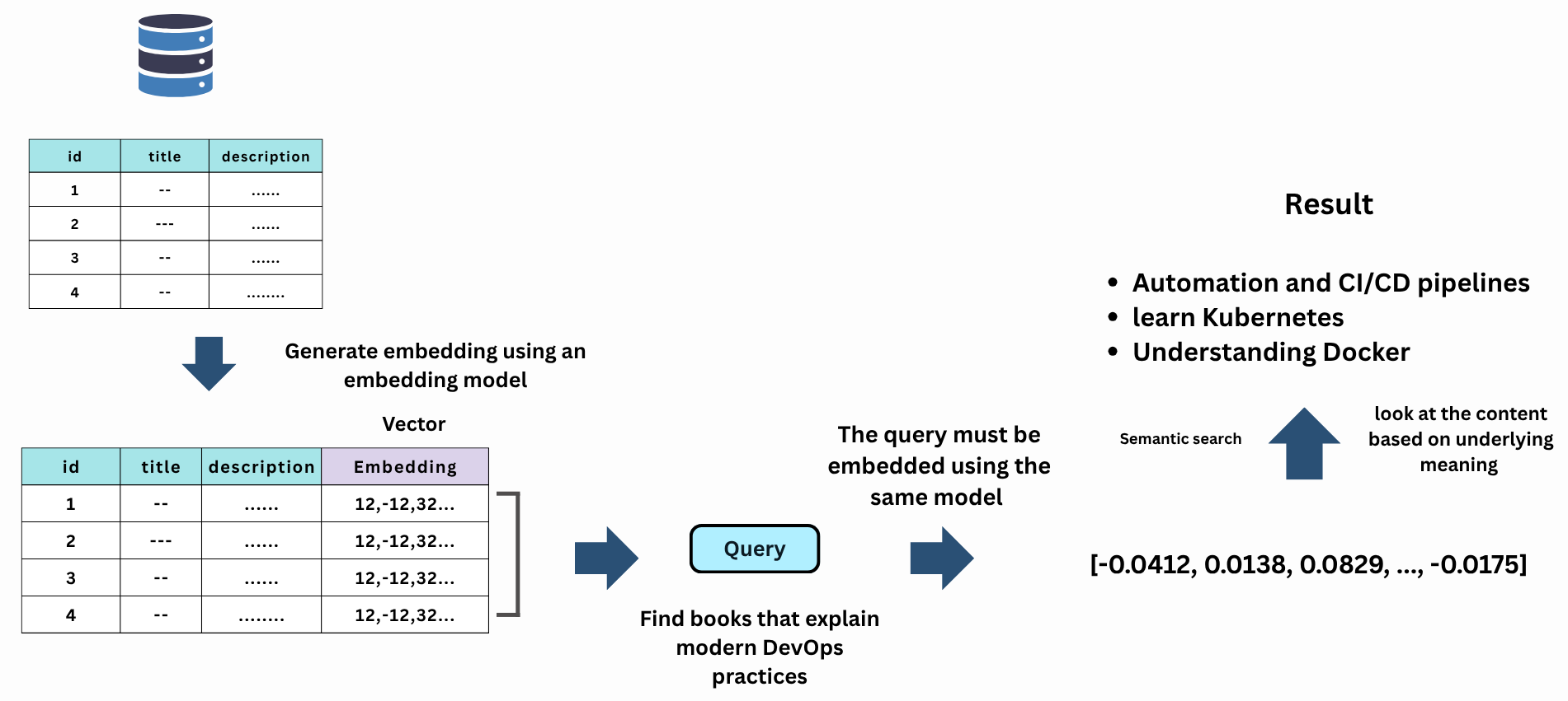
This limitation led to the emergence of new approaches to data representation, where information is expressed not as text or categories, but as mathematical vectors in a multidimensional space.

What is Vector
A vector is a mathematical representation of data as an array of numbers, essentially a point in an n-dimensional space. Each dimension represents a feature or characteristic of the data.
Vectors are used widely in mathematics, machine learning, and artificial intelligence to represent complex objects such as Text, Images, Audio, and Video.
For example, a sentence can be converted into a vector (a list of numbers) using an embedding model. Each number in the vector captures some aspect of the sentence’s meaning or context. This allows computers to compare pieces of text based on semantic similarity, not just matching keywords.
When Databases and Vectors Come Together
At first glance, it might seem that any database capable of storing numerical arrays or JSON data can store vectors. While that’s technically true, simply storing vectors doesn’t make a database a vector database.
A true vector database goes beyond storage; it provides specialised capabilities such as:
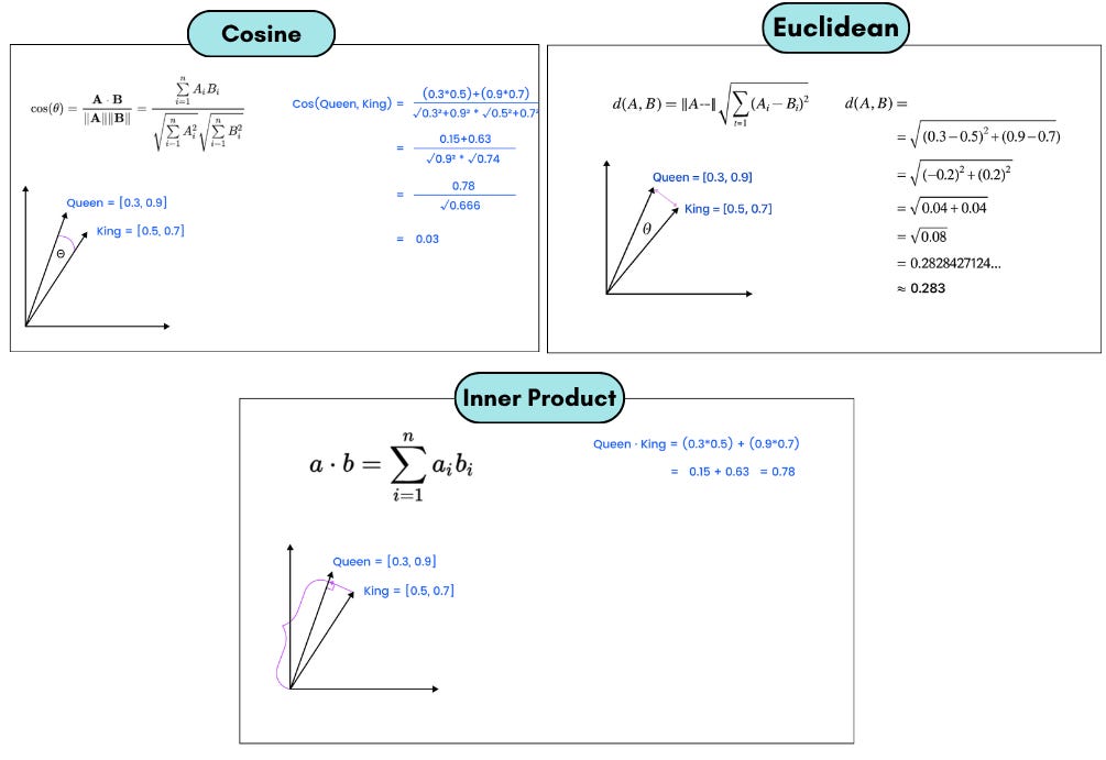
Vector similarity search: Finding the most similar vectors to a given input using distance metrics like Cosine similarity or Euclidean distance, or Inner Product.

Efficient indexing: Using algorithms such as HNSW (Hierarchical Navigable Small World) or IVF (Inverted File Index)3 to speed up searches across millions or billions of high-dimensional vectors.
Optimised storage: Handling large-scale, high-dimensional data efficiently.
Metadata association: Storing and querying metadata linked to each vector (e.g., document IDs, titles, timestamps).
These features enable powerful use cases such as:
Searching for visually similar images.
Finding related documents or products.
Powering recommendation systems.
Enabling retrieval-augmented generation (RAG) for LLMs and so on.
6 Key Concepts Behind Vector Databases
Embedding
To make similarity search possible, we must first convert the data into a numerical form, known as vectors. Embedding models4 perform this conversion.
An embedding5 is a numerical representation of data (text, image, or audio) in a multi-dimensional vector space. Embedding models are trained to capture the semantic meaning or context of the data.
In simple terms, embedding models take raw data and translate it into numbers in such a way that similar meanings produce similar vectors, a process known as vectorisation.
Example:
An embedding model might map:
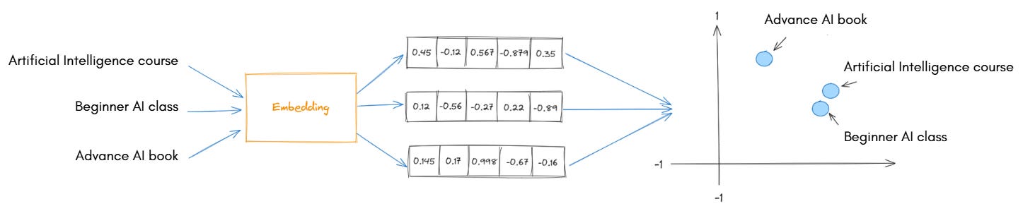
“Artificial Intelligence course”“Beginner AI class”
to two vectors:
[0.8, 0.1, 0.9, 0.4, 0.2][0.7, 0.2, 0.85, 0.35, 0.25]
that are close to each other in vector space because they have nearly the same meaning.
These embeddings preserve semantic relationships, meaning that related words, sentences, or images will have vectors located near each other.
Note: A database computes similarity to find the closest one. Most vector databases support cosine similarity, Euclidean distance, or inner product natively.
Dimentonality
In vector databases, dimensionality is a key concept.
Dimensionality refers to the number of components (or features) that make up a vector, in other words, the length of the vector. Each number in the vector represents a specific attribute or feature of the data.
As programmers, we can think of a vector as a simple array of numbers, where the size of the array corresponds to its dimensionality.
We might wonder: why not just one number per vector?
Think of describing a student:
Using just one number (e.g., height) isn’t enough.
To fully describe the student, we also need to consider their weight, age, GPA, and other relevant attributes.
The same principle applies to words, sentences, or documents. A single number cannot capture all aspects of meaning. By using many numbers, embeddings can encode nuances and context.
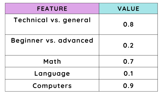
Example: An embedding vector might have dimensions that represent:
Whether the topic is technical or general.
Whether the content is beginner-level or advanced.
Whether it relates to math, language, or computers.
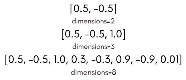
For instance, a 5-dimensional example vector could look like this:
By using hundreds of dimensions, embeddings can capture detailed differences between data points.
It’s worth mentioning that choosing dimensionality is a trade-off:
Higher dimensionality: captures more detailed meaning and small differences between data points.
Lower dimensionality: uses less memory and is faster to compute.
By carefully selecting dimensionality, we can balance accuracy, efficiency, and scalability, ensuring our vector-based applications perform well both technically and for business needs.
Note: When comparing embedding models, one of the key details we look at is their number of dimensions.
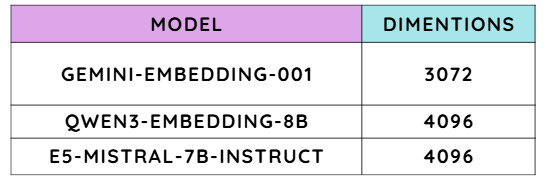
“If you’d like to explore more about embedding models and their characteristics, check out the MTEB leaderboard on Hugging Face.”
Chunking
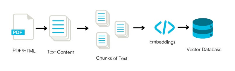
Chunking is the pre-processing step of splitting large texts into smaller pieces of text, called chunks.
We already know that a vector database stores objects as vectors to capture their meaning. But how much text does each vector represent?
That’s exactly what chunking defines: each chunk is the unit of information that gets vectorised and stored in the database.
Consider a case where the source text is a set of books. A chunking method could split the text into chapters, paragraphs, sentences, or even individual words, each treated as a separate chunk.
Although conceptually simple, chunking can greatly impact the performance of vector databases and enhance output quality, particularly when applied alongside foundation models.
For example, course descriptions can be long. If we store them as one large block, the embedding becomes too broad, making searches less precise. Instead, we break them into smaller, meaningful chunks.
However, splitting too aggressively can break the context:
Chunk 1: “…students will learn supervised…”
Chunk 2: “…and unsupervised learning methods…”
If we search for “unsupervised learning”, we might miss it because the phrase was split across chunks.
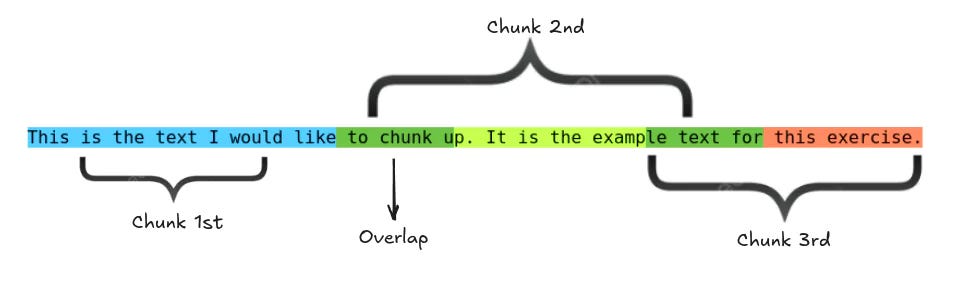
To prevent this, we use overlap, repeating a few words between chunks. Overlap keeps context intact so that searches return more accurate and meaningful results.
Scoring (Similarity Scoring)
A similarity score tells us how close two vectors are in the vector space:
High score: vectors are close.
Medium score: somewhat close.
Low score: far apart.
Example
Suppose a student searches for “Beginner AI class” and we compare it to several courses:
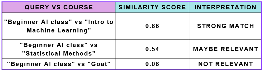
We could set a threshold, e.g., 0.7, to return only items above that score. This ensures that very irrelevant results are ignored.
However, a high similarity score doesn’t always mean two items are truly related; vectors may be close due to shared words or patterns rather than actual meaning. That’s why we often apply a ranking step after similarity scoring.
Ranking
Absolute similarity scores can vary depending on the embedding model, data domain, or normalisation method. Because of this, relying solely on a fixed threshold may not always be ideal.
Ranking offers a more flexible and robust approach:
Instead of filtering results with a strict cutoff, sort all items by their similarity scores in descending order.
Then, return the top N results, even if some scores fall below your usual threshold.
Example:
Query results:
Course A: 0.52
Course B: 0.49
Course C: 0.48
If the threshold were 0.7, no results would be returned.
However, ranking ensures users still receive the most relevant results available:
Top 2 ranked courses:
Course A (0.52)
Course B (0.49)
This approach guarantees that users always see the best available matches, even when similarity scores are relatively low or inconsistent.
It’s also the foundation for more advanced techniques like re-ranking, which refine results further using metadata, user signals, or machine learning models.
Search Modes
It’s important to understand how a vector database retrieves results.
Most modern systems support three primary search modes, each with its own strengths and trade-offs: