SQL Behind the Curtain: How Are Queries Executed?

Explore the journey of our SQL query guided by execution plans

Nov 19, 2024

∙ Paid

Imagine our SQL query is like a treasure map, and the database is a huge area to explore. The execution plan is like a detailed route created by an expert navigator (the SQL engine) to help us find the treasure (our query results) as quickly as possible. Understanding this route lets us spot shortcuts, avoid wrong turns, and reach our goal faster.

By understanding SQL execution plans and the basics of Big O notation, we can optimise our queries to be faster and more effective.

In this post, we will explore how SQL Queries are executed behind the scenes.

What is Big O Notation?

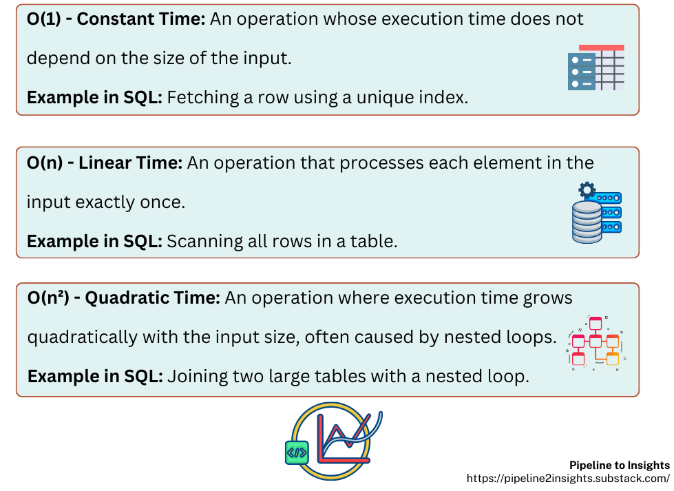
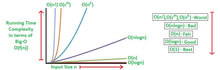
Big O notation describes the performance of an algorithm in terms of how it scales with the size of the input. It provides a high-level understanding of the time or space complexity, helping us evaluate the efficiency of different operations.

From: “https://www.geeksforgeeks.org/analysis-algorithms-big-o-analysis/”

While we don’t need to be a computer scientist to write SQL, knowing the relative costs of operations helps when optimising queries.

How does an SQL query execute step by step?

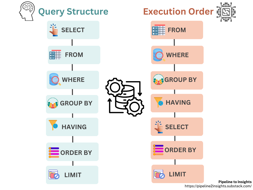
SQL queries are not executed in the order they’re written. Instead, an SQL engine transforms our query into actionable steps through the following process:

Parsing: The engine breaks the query into components like keywords (SELECT, FROM), identifiers (table/column names). operators (=, >, etc.), validating syntax, and semantics to produce a parse tree.
Query Transformation: The parse tree is translated into relational algebra, and multiple logical query plans are generated to explore various execution strategies.
Optimisation: The optimiser evaluates these plans, choosing the most efficient one by considering factors like indexes, join types, and table statistics. This results in an execution plan that guides how data will be retrieved and processed.
Execution: The database engine carries out the execution plan step by step, fetching, filtering, grouping, and sorting data as specified in the query.

Let’s say we have a table named sales with the following structure:

CREATE TABLE sales (
    sale_id SERIAL PRIMARY KEY,
    product_id INT,
    customer_id INT,
    sale_date DATE,
    sale_amount NUMERIC
);

Now, we want to query total sales for a specific product, and if we run this query:

EXPLAIN ANALYZE
SELECT SUM(sale_amount)
FROM sales
WHERE product_id = 42;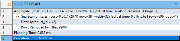

The output above shows how the SQL engine processed the query step by step:

Aggregate: The engine calculated the total sales (SUM(sale_amount)) for rows where product_id = 42. This step took 6.745 ms to complete.
Seq Scan: A sequential scan was performed on the sales table because no index was available for product_id. The engine scanned all 100,000 rows, filtering out 99,004 rows that didn’t match the condition.
Filter: The condition product_id = 42 was applied during the scan to identify the 996 rows that matched.
Planning Time: The query planner took 0.085 ms to generate the execution plan.
Execution Time: The total execution time for the query was 6.765 ms.

Understanding these steps helps us write queries that work well, reducing resource usage and improving speed.

Combining Big O Notation and Execution Plans

Here’s how we can use Big O notation alongside execution plans to optimise our queries:

Indexes Matter: Indexing can reduce the complexity of searches from O(n) (scanning the whole table) to O(log n). Use indexes for frequently queried columns.
Join Smarter: Nested loops can be costly (O(n²)) if the dataset is large. Consider using hash joins or merge joins, depending on the database and data size.
Filter Early: Push conditions into the WHERE clause to reduce the data processed in later stages.
Analyse Plans: Use tools like EXPLAIN (PostgreSQL, MySQL), or AUTOTRACE (Oracle) to identify bottlenecks in our query.

Putting Theory into Practice

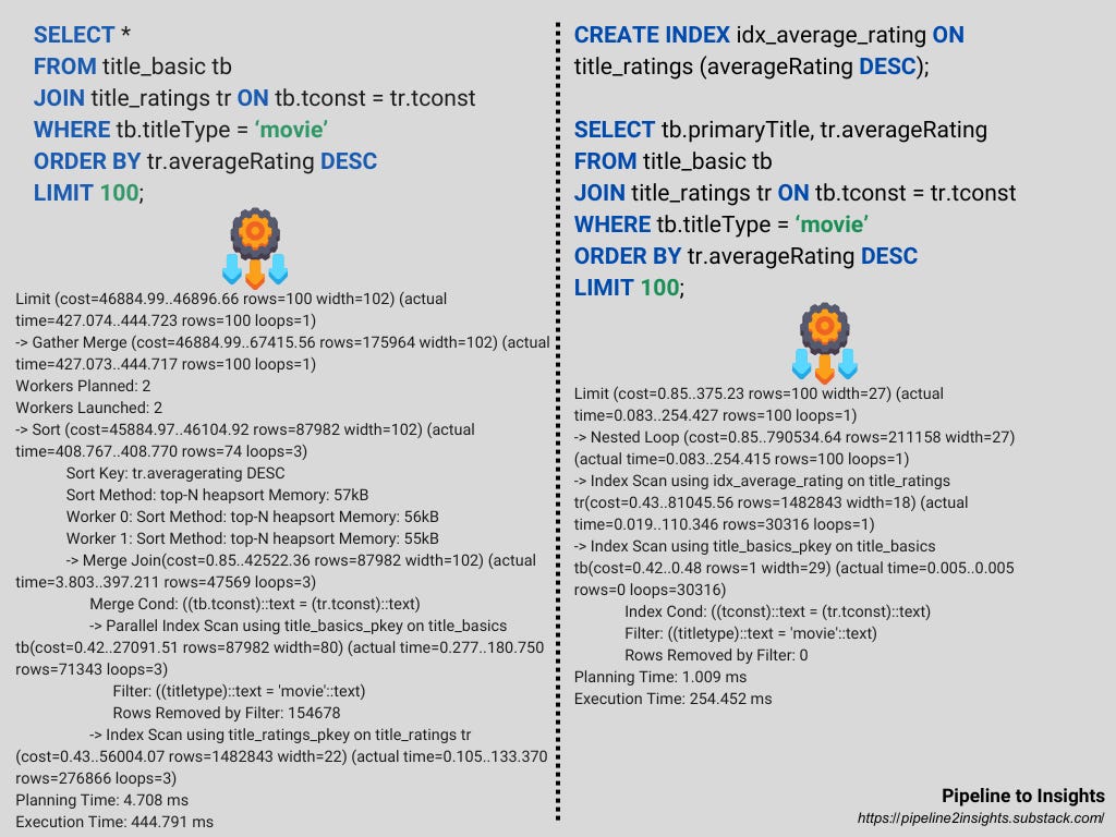
To illustrate the impact of Big O notation and execution plans on query performance, consider two versions of a query that retrieves the top-rated movies.

Key Differences

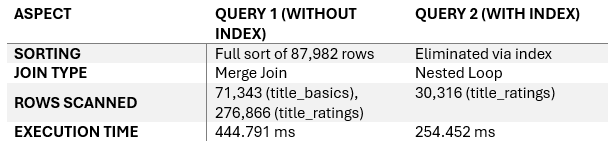
Indexes Eliminate Expensive Sorting: Query 2 leverages the index on averageRating to avoid a full sort, significantly reducing execution time.
Efficient Join Strategies: Query 2 uses a Nested Loop with indexed scans, processing fewer rows compared to Query 1’s Merge Join.
Reduced Data Volume: Query 2 processes fewer rows overall, focusing only on relevant data, making it ~43% faster than Query 1.
Practical Insight: Adding indexes on frequently sorted or filtered columns is a simple yet impactful way to optimise query performance.

Pipeline To Insights