
Week 5/31: Data Modelling for Data Engineering Interviews (Part #2)
Week 5 of 33-Week Data Engineering Interview Guide

In this post, we explore common data modelling interview topics by solving interview questions, including:
Normalised Forms
Types of Slowly Changing Dimensions (SCDs)
Differences between the Kimball and Inmon approaches
The concept of "One Big Table"
Additionally,
We solve a case study on converting data tables into 3NF form.
We solve a case study on SCDs and Star Schema.
We share resources for a mock Airbnb data modelling interview to help you practise.
In the first post of this series, we covered key concepts such as:
Definitions of data modelling
Types of data models
ER diagrams
Distinctions between OLTP and OLAP systems
If you haven’t already, check out the post below for a strong foundation:

Importance of Data Modelling Interviews

Data modelling interviews assess a data engineer’s ability to turn business needs into effective data solutions. Success requires both technical expertise and strong communication skills. During these interviews, asking clarifying questions can provide additional context, as interviewers often reveal more details during discussions.
Question 1
Case Study: Normalising Data to 3NF
Identify the current form of the given data and normalise it to 3NF.
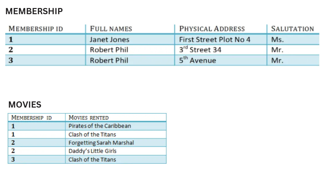
We are provided with the above tables. We start by identifying their current form (e.g., 1NF, 2NF, 3NF). If the tables are not in 3NF, we explain the steps to normalise them.
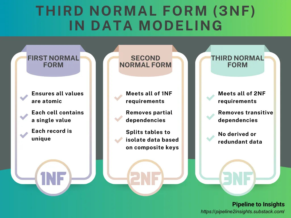
To answer effectively, let’s remember the rules:
1NF:
All values must be atomic.
Each cell contains a single value.
Each row is unique.
2NF:
Satisfy all 1NF rules.
All data must depend on the primary key. Columns not dependent on the primary key should be moved to separate tables.
3NF:
Satisfy all 2NF rules.
The primary key must fully define all columns, and no column should depend on any other non-primary key.
Checking the Membership Table:
Original Table
This table meets 1NF and 2NF rules.
The
MEMBERSHIP IDdetermines theFULL NAMESandPHYSICAL ADDRESS.However, the
FULL NAMESandPHYSICAL ADDRESSdon’t depend on any other key.Salutations are not determined by the
MEMBERSHIP ID, violating 3NF rules.
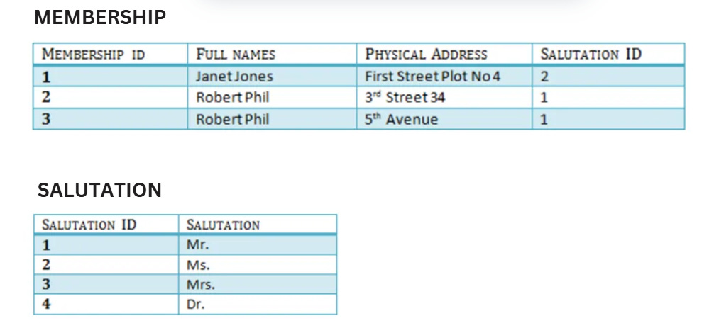
Normalisation Steps
Create a new table for salutations.
Ensure the original table only contains columns that fully depend on the primary key.
Final Structure
A normalised table in 3NF with clear relationships to supporting tables (e.g., Salutations).
Checking MOVIES table:
Original Table
This table meets 1NF, 2NF and 3NF rules.
Normalisation Steps
The requirement only extends up to 3NF, so there’s no need to go beyond that level of normalization.
Final Structure
No structure change is required.
Tip: We suggest having the below visual in your pocket as a normal forms reference.
Question 2
What is the impact of data modelling on data storage and scalability?

Answer (Direct):
Data modelling defines the structure and organisation of data, which has a significant impact on storage and scalability.
Effective data modelling:
Reduces storage requirements by eliminating redundant data.
Improves data retrieval efficiency, enabling faster and more reliable access to information.
Enhances scalability, allowing systems to handle increasing data volumes without performance degradation.
Supports system flexibility, enabling changes or updates to be implemented without affecting existing operations.
Tip: Sometimes it is better to explain things by using metaphors it helps explaining them clearly while allowing us to showcase our understanding.
Alternative Answer (with Metaphors):
Data modelling is like creating a blueprint for how your data is organized. Good data modelling helps you:
Save storage space by eliminating data redundancy.
Access and retrieve data quickly and efficiently.
Scale your system seamlessly as data volume grows.
Implement system changes without disrupting existing functionality.
Think of it like organising a library, when books are well-categorised and clearly labelled, it's easier to store them efficiently, find what you need, add new books, and reorganise sections when needed.
Question 3
What is a Surrogate Key?
A surrogate key is a unique, artificial identifier used in a data warehouse. It's typically a simple number, automatically generated by the system, that joins data between tables. Unlike natural keys, which can change when systems are modified, surrogate keys remain consistent and independent, ensuring data warehouse stability. These keys simplify data processing, boost performance, prevent issues with changing data, and make it easier to manage complex table relationships.
Question 4
Explain slowly changing dimensions and how to model them.
Slowly Changing Dimensions (SCDs) handle changes in dimension data over time, ensuring accurate historical tracking and reporting. There are six common types of SCDs, each suited for different requirements. Below is an explanation of each type using a Customer Dimension for a retail business as an example.
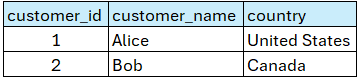
Type 0 – Fixed Dimension
No changes are allowed; the data remains static.
Example: A customer's assigned country remains the same as the one they signed up from, regardless of future relocations.
Use Case: When historical integrity is critical, and changes must not affect existing reports.
Example:
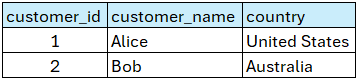
Type 1 – No History
Updates overwrite existing data, with no historical tracking.
Impact: All related fact records are now associated with the updated value, regardless of when they were created.
Use Case: When historical tracking is not required, and only the latest information matters.
Example: If Bob moves to Australia, his country attribute is updated to “Australia” and previous country information is lost.
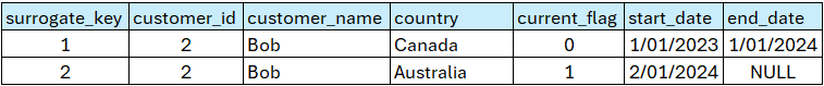
Type 2 – Row Versioning
Changes are tracked by creating new rows for each update, along with metadata to indicate current and historical versions.
To implement Type 2, we need to add the following columns:
Surrogate Key: A unique ID for each version of the record.
Current Flag: Indicates whether the record is the current version.
Start Date: The date when the record became active.
End Date: The date when the record was replaced.
Use Case: When maintaining a full history of changes is essential.
Example: When Bob moves, a new record is created with updated details, and the previous record is marked inactive.
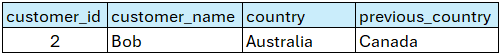
Type 3 – Previous Value
A new column is added to store the previous value of the changing attribute.
Limitations: Only one prior value is stored, so multiple changes (e.g., Bob moving twice) require additional columns or result in data loss.
Use Case: When limited historical tracking is sufficient.
Example: Add a “Previous Country” column to track Bob’s last country.
Type 4 – History Table
Changes are tracked in a separate history table, while the current value remains in the dimension table.
Dimension Table: Contains the latest customer details.
History Table: Stores all previous versions of the record.
Use Case: When separating current and historical data simplifies querying and reporting.
Example: Bob’s moves are tracked in a history table while the current table reflects his latest country.


Type 6 – Hybrid (Types 1, 2, and 3 Combined)
Combines elements of Types 1, 2, and 3 to provide both historical data and current snapshots.
Features:
Tracks all changes using row versioning (Type 2).
Maintains a “Current Value” column (Type 1).
Adds a “Previous Value” column (Type 3).
Use Case: When both comprehensive historical tracking and easy access to the latest data are required.
Example: A single model tracks Bob’s complete history, his current country, and his previous country.

Question 5
What are the differences between normalisation and denormalisation in data modelling, and when should each approach be used?
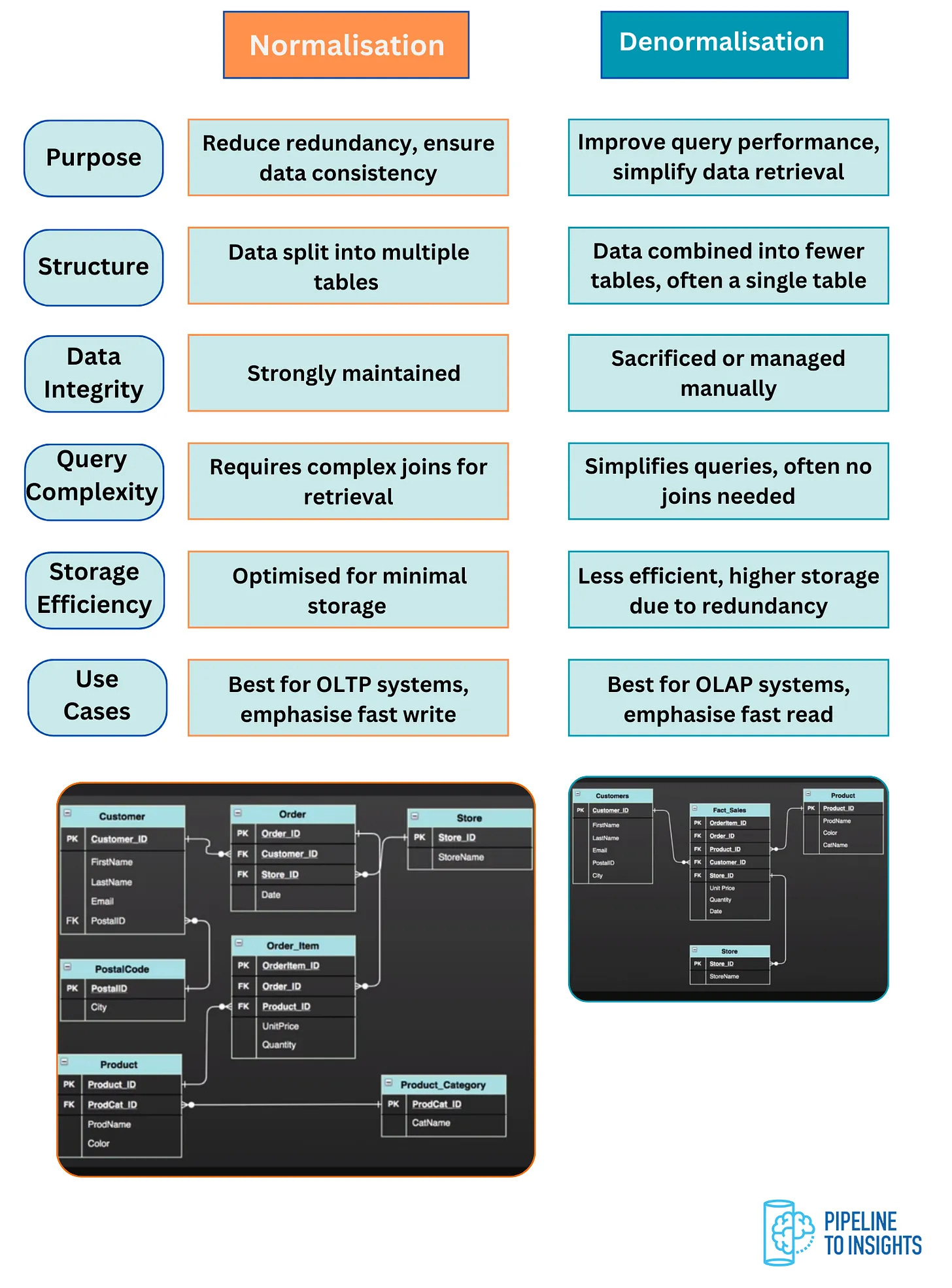
Normalisation and denormalisation are two contrasting approaches in data modelling, each serving distinct purposes based on the system's goals.
Key Differences
Purpose:
Normalisation: Reduces redundancy and ensures data consistency by splitting data into multiple related tables.
Denormalisation: Combines data into fewer tables to improve query performance and simplify data retrieval.
Structure:
Normalisation: Breaks data into smaller, logically related tables.
Denormalisation: Merges related data into larger, often single tables.
Data Integrity:
Normalisation: Strongly maintains data integrity by avoiding redundancy.
Denormalisation: May sacrifice some data integrity for performance gains, with manual or system-managed consistency.
Query Complexity:
Normalisation: Requires complex joins to retrieve data, which can slow down read operations.
Denormalisation: Simplifies queries as fewer joins (or none) are needed, leading to faster read operations.
Storage Efficiency:
Normalisation: Optimised for minimal storage by eliminating redundancy.
Denormalisation: Requires higher storage due to data duplication, as seen in the denormalised schema example.
Use Cases:
Normalisation: Best suited for OLTP (Online Transaction Processing) systems, where fast writes and data consistency are crucial.
Denormalisation: Ideal for OLAP (Online Analytical Processing) systems, focusing on fast reads and simplifying analytics.
The choice between normalisation and denormalisation depends on the system’s priorities:
Opt for normalisation in transactional systems where data consistency and storage efficiency are priorities.
Choose denormalisation for analytical systems where query performance and simplicity are more important.
Tip: We suggest having the below visual in your pocket as a normalisation vs. denormalisation reference.
Question 6
What are the differences between the Kimball and Inmon approaches to data warehousing?
The Kimball and Inmon approaches represent two widely used methodologies for building and managing data warehouses. Both have their strengths and weaknesses, and the choice depends on the specific requirements of the organisation.
Kimball Approach: Bottom-Up Methodology
Process:
Begins by creating data marts tailored to specific business needs.
These data marts are sourced from OLTP systems and later integrated into a centralised data warehouse using a denormalised star schema.
Key Characteristics:
Focuses on speed to value with faster ROI.
Prioritises scalability and flexibility by allowing individual teams to implement data marts independently.
The use of star schemas simplifies querying for business analysts and report generation.
This may lead to challenges in creating reusable structures and maintaining consistent ETL processes as the system grows.
Best Suited For:
Organisations need quick insights and immediate business value.
Environments with smaller-scale or decentralised teams.
Inmon Approach: Top-Down Methodology
Process:
Starts with a centralised data warehouse built in 3NF, sourced directly from OLTP systems.
Data marts are created from the data warehouse as needed, also maintaining a 3NF structure.
Key Characteristics:
Emphasises a structured and consistent design from the outset.
Ensures easier maintenance and facilitates long-term scalability.
Better suited for advanced use cases like data mining and enterprise-wide analytics.
Takes more time and resources to implement compared to the Kimball approach.
Best Suited For:
Large organisations with complex data ecosystems.
Scenarios where a structured and unified view of enterprise data is critical.
Comparison Analogy
Kimball (Bottom-Up): Imagine starting with small, independent sections like book inventory or borrowing history (data marts) and eventually combining them into a larger library system (data warehouse). This approach provides quicker access to actionable insights but can pose challenges in maintaining consistency and integration over time.
Inmon (Top-Down): Think of building a single, detailed master catalog (data warehouse) first, then creating smaller sections (data marts) for specific purposes. While this approach takes longer to set up, it ensures a more robust and consistent foundation.
Choose Kimball: For quick, flexible implementations where time-to-value is a priority.
Choose Inmon: For structured, long-term solutions that require consistency and maintainability.
Many organisations adopt a hybrid approach, combining the strengths of both methodologies to balance flexibility with structure.
Question 7
What are the differences between the Star Schema and the Snowflake Schema?
The Star Schema and Snowflake Schema are two widely used designs for organising data in a data warehouse. Both have their strengths and are chosen based on the specific needs of the system.
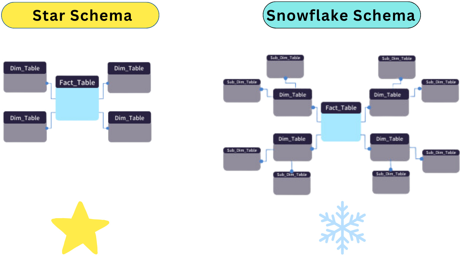
Star Schema
Structure:
The Star Schema features a central fact table surrounded by multiple dimension tables, creating a star-like design.
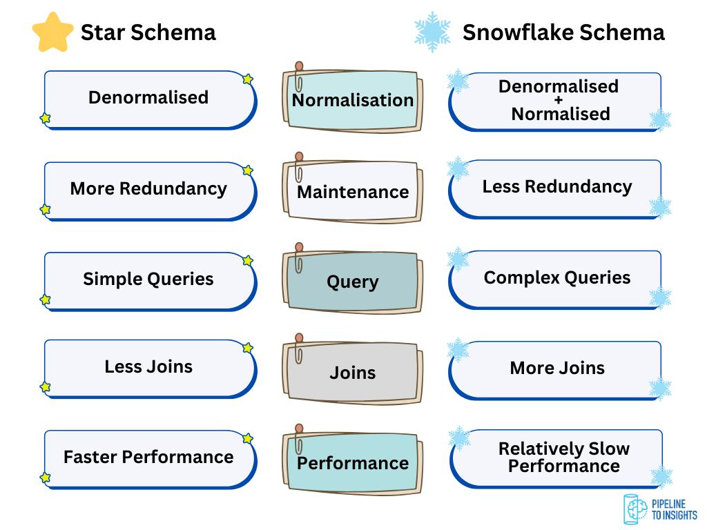
Dimension tables are denormalised, meaning they contain all descriptive attributes directly, without additional hierarchy levels.
Key Characteristics:
Simple and intuitive structure, making it easy to understand and query.
Ideal for business intelligence and reporting tools that perform straightforward queries.
Requires more storage space due to denormalisation, as there is some duplication of data in dimension tables.
Offers faster query performance since fewer joins are needed.
Use Cases:
Best suited for OLAP systems where simplicity and query performance are prioritised.
Snowflake Schema
Structure:
The Snowflake Schema also centres around a fact table but normalises dimension tables by splitting them into smaller, related tables.
This results in a schema that resembles a snowflake, with dimension tables branching into additional layers of tables.
Key Characteristics:
More complex and requires more joins for queries due to higher normalisation.
Reduces data redundancy and optimises storage efficiency.
Queries may perform slower compared to the Star Schema, as multiple joins are required to retrieve data.
Better suited for environments where maintaining data integrity is crucial.
Use Cases:
Suitable for large, complex data warehouses where storage optimisation and data integrity are important.
Tip: We suggest having the below visual in your pocket as a star schema vs. snowflake schema reference.
Question 8
What is the One Big Table (OBT) approach in data modelling, and when should it be used?
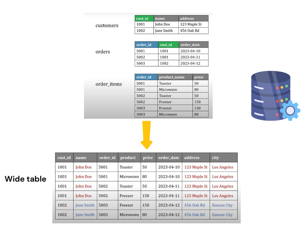
The One Big Table (OBT) approach is a denormalised data model that consolidates multiple tables, both facts and dimensions into a single, large table. It is commonly used for reporting and analytics, especially in scenarios where query performance is a higher priority than strict data normalisation.
Key Features
Denormalised Structure:
All data is stored in a single table, including both facts and dimension attributes.
This leads to data redundancy, as attributes from dimension tables are repeated for each related fact.
Faster Query Performance: Since all data resides in one table, queries can be executed faster without requiring joins, making it well-suited for analytical workloads.
Eliminates Joins: Simplifies query writing by removing the need for complex joins between multiple tables.
Increased Storage Requirements: The redundancy inherent in a denormalised structure results in higher storage consumption compared to normalised models.
Potential Data Integrity Issues: The absence of normalisation can lead to inconsistencies during updates or changes, as redundant data must be managed manually.
Why Use the One Big Table Approach?
Optimised for Analytics:
The OBT model prioritises query performance, making it ideal for environments where quick data retrieval is critical.
It is particularly effective for large datasets in reporting scenarios, where the need for speed outweighs concerns about storage or data integrity.
Simplified Queries:
Reduces the complexity of queries, making it accessible for business users or analysts who may not have advanced SQL skills.
Use Cases
High-Performance Reporting: Dashboards or reports that require fast responses from analytical queries.
Data Lakes and Warehouses: Scenarios where data is loaded for read-heavy analytics with minimal updates.
Prototyping: Quick prototypes for analytics and reporting when query performance is a priority.
Question 9
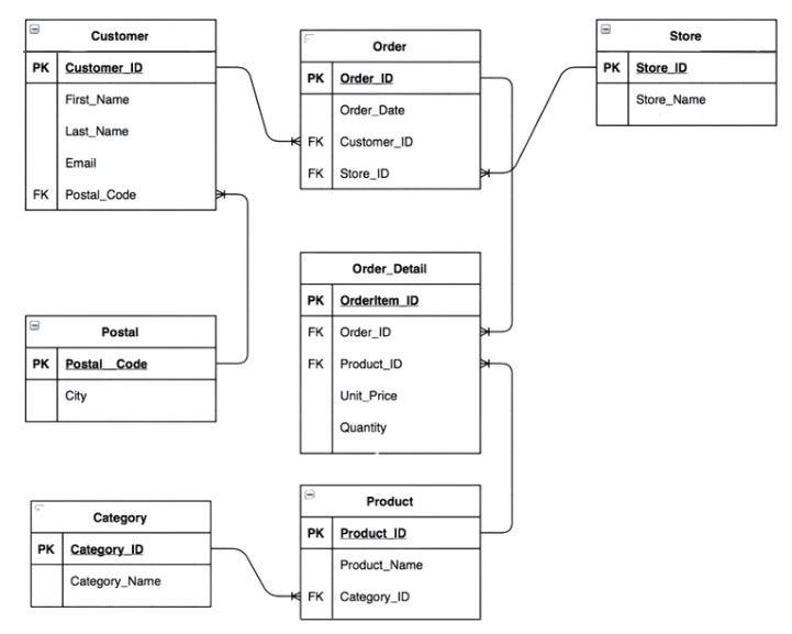
Case Study: Create a Dimensional Model for a Retail Business using Star Schema
A company produces products such as electronics (phones, tablets) and beauty items (perfumes, lipsticks). Customers shop at nearby stores, often purchasing a mix of products in a single visit, recorded on one invoice.
The company needs a data warehouse optimised for fast-read operations and complex queries, transforming the existing 3NF OLTP model into a dimensional model using the Star approach.
Additional Information:
A specific store sells multiple products daily to various customers.
The business objective is to track how many products are purchased by a customer at a single store.
Solution
1. Identify the Business Objective
The purpose of the dimensional model is to support analytics by storing information about the number of products purchased from a single store by a customer.
Tip: Before assuming, always ask clarifying questions to refine the objective.
2. Determine the Granularity
Granularity refers to the level of detail in the fact table.
In this scenario, the granularity is at the level of Product, Date, Store, and Customer.
Considerations:
Too Detailed: This leads to a massive database that is harder to manage.
Too Broad: Limits meaningful analysis.
If unsure, always seek clarification from the interviewer.
3. Define Dimension Tables
Dimensions provide descriptive attributes about the facts and are linked to the fact table via foreign keys.
Key Dimensions for This Case:
Product: Attributes include product_id, product_name, category, and brand.
Customer: Attributes include customer_id, customer_name, and location.
Store: Attributes include store_id, store_name, and region.
Date: A separate date dimension is required to track daily sales.
Guidelines for Dimension Tables:
Logical Belonging: Attributes should belong to the same entity (e.g., city and region for store location).
Strong Relationships: Attributes should have one-to-many relationships.
Hierarchy: Attributes like product and product group should follow a natural hierarchy.
Naming Convention: Prefix dimension tables with
dim_(e.g.,dim_customer).Simplification: Denormalise where possible by merging related attributes (e.g., include category name directly in the product dimension).
4. Define the Fact Table
The fact table stores measurable metrics and foreign keys referencing dimension tables.
Metrics to Include:
total_sales: Total revenue for the sale.
unit_price: Price per unit of the product.
quantity: Number of units sold.
Primary Key:
Instead of using a composite key (combination of product_id, customer_id, store_id, and date_id), create a system-generated surrogate key,
sales_id, to uniquely identify each record.
5. Add Surrogate Keys
Surrogate keys ensure consistency and uniqueness across dimension tables.
For the fact table, a surrogate key like
sales_idsimplifies joins and ensures efficient query performance.
6. Validate Relationships
Validate the one-to-many relationships between dimension tables and the fact table:
Dimensions: Product, Store, Customer, and Date tables are on the "one" side.
Fact Table: On the "many" side, a single product, store, or customer can have multiple sales records.
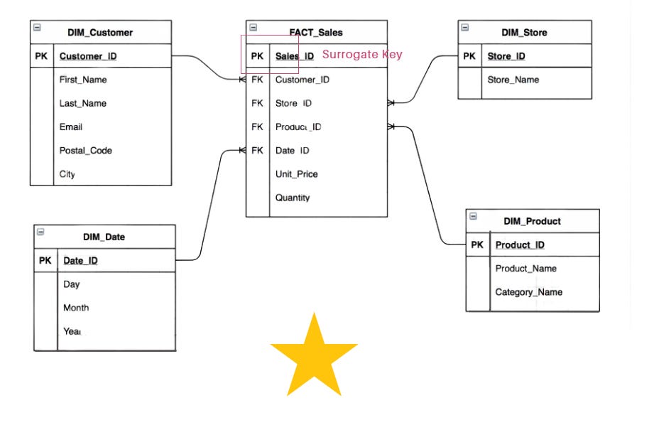
Final Dimensional Model
Dimension Tables:
dim_productdim_customerdim_storedim_date
Fact Table:
fact_sales
Additional Practice
Mock Interview by Airbnb: [Link]
Real-time Data Modeling & System Design Mock Interview for Data Engineers:[Link]
Conclusion
In this post, we explored commonly asked data modelling questions in interviews, covering key topics such as:
3NF (Third Normal Form) and its relevance in database design.
Slow-Changing Dimensions and Strategies for Handling them.
Star Schema vs. Snowflake Schema, their design patterns, and use cases.
The One Big Table (OBT) approach and its practical applications.
Real-world case studies showcasing practical data modelling scenarios.
Additionally, we provided resources for a mock Airbnb data modelling interview to help you practice and refine your skills.
If you want to dive into the details of;
Normalisation vs Denormalisation
Third Normal Form (3NF)
Dimensional Modelling
Check out the post below for more details.

Also for the full plan of our Data Engineering Interview Preparation Guide, please check the below post.

Stay tuned for our next post, where we’ll dive into Data Vault modelling, a technique gaining popularity, especially in enterprise-level companies!
We Value Your Feedback
If you have any feedback, suggestions, or additional topics you’d like us to cover, please share them with us. We’d love to hear from you!